We graph complicated formulae to develop an understanding of the characteristics of these functions. Since the goal of computing is insight, we desire our graphing systems to be both correct and complete. By correctness we mean that the points plotted do lie on the graph and that features visible in the plot such as extrema, crossings, and asymptotic behavior are actually part of the graph. By completeness we mean that all such features of the graph are visible in plot. All systems we examined fail to meet these criteria by both errors of omission - failing to plot significant features of the graph, and errors of commission - displaying features which are artifacts of the graphing algorithm having nothing to do with the mathematical surface.
     In our discussion of related works, 1+x²+0.0125ln|1-3(x-1)| demonstrates a typical error of omission; the plot leaves out an important feature of the curve. Figure 1 and 2 demonstrate errors of commission where structure visible in the plot is just an artifact of the graphing algorithm.

Discontinuities

     Consider the criterion that the points rendered actually lie near the surface. All systems we examined given z=tan^-1x/y will produce an image similar to Figure 6a.
     The vertical polygons along the x-axis do not belong to the graph. This is not a problem of under sampling. Choosing a denser sampling would not help; nor would adaptive sampling. The problem is that although the function is evaluated correctly at each point sampled, the function is not continuous. Hence, connecting the computed points with polygons in 3D or with lines 2D adds points to the image which do not belong to the graph. Maple V.3 includes an option (discont=true) to 2D plotting which symbolically solves to find discontinuities in the function and does not connect the points across a discontinuity. However, this option is not available for 3D plotting.
     To improve on this, one can compute interval bounds on the partial derivatives to get an interval bound on the normal vector. The normal vector of a polygon across a discontinuity could be rejected if it is not contained in this interval bound. Figure 6 shows z=tan^-1x/y rendered both in the shipping Graphing Calculator and also in an experimental version performing this surface normal test automatically.

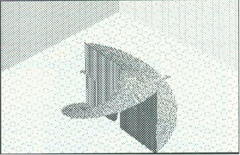
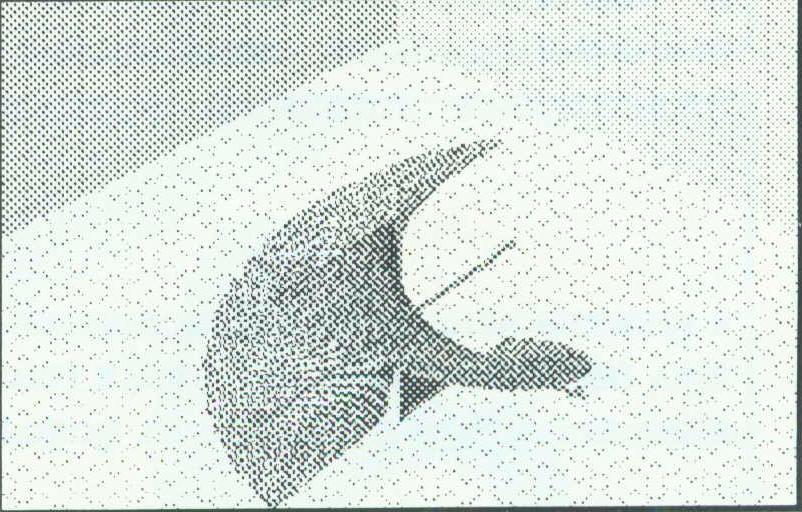
Figure 6: tan^-1x/y with and without the surface normal test

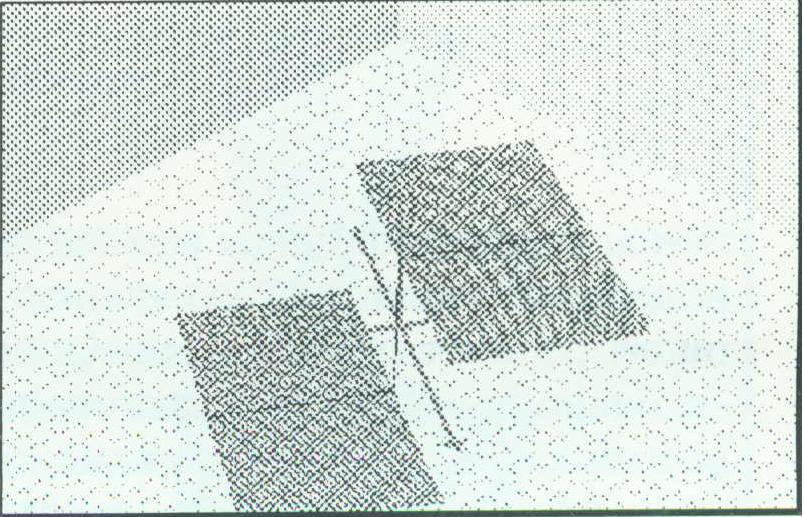
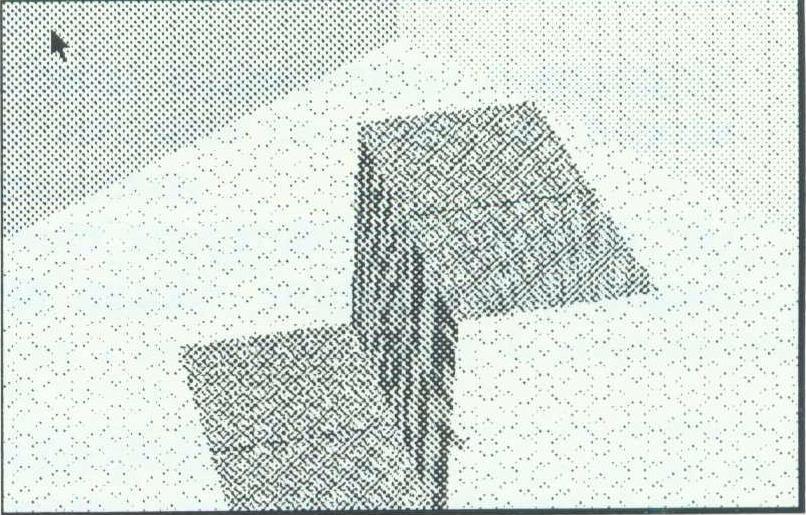
Figure 7: z = | x |/x and z=tanh (1000x) using the surface normal test

     Consider now z=|x|/x, and z=tanh(1000x). By choosing a sufficiently large constant, these surfaces can be made arbitrarily close. A naive algorithm which samples the function will not distinguish them. By using this surface normal test together with an otherwise naive 3D renderer, an experimental version of the Graphing Calculator produced Figures 7a for z=|x|/x, and 7b for z=tanh(1000X). The correctness of these plots relies on being able to compute bounds on the partial derivatives of the function, ignoring points where the partial derivative is undefined. Naively following the chain rule symbolically differentiating the expression, and simplifying the result satisfies this. For example, we do not display the vertical facet around x=0 for |x|/x simply bacause the x-component of its normal vector would not belong to the interval [0..0] which is the interval bound of the derivative of |x|/x (assuming d(|x|/x)/dx simplifies to 0, rather

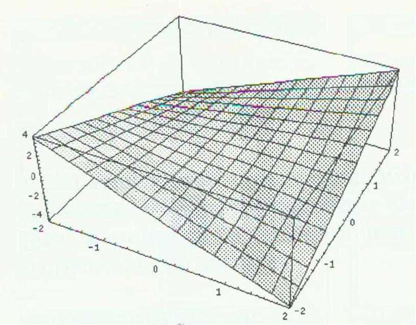
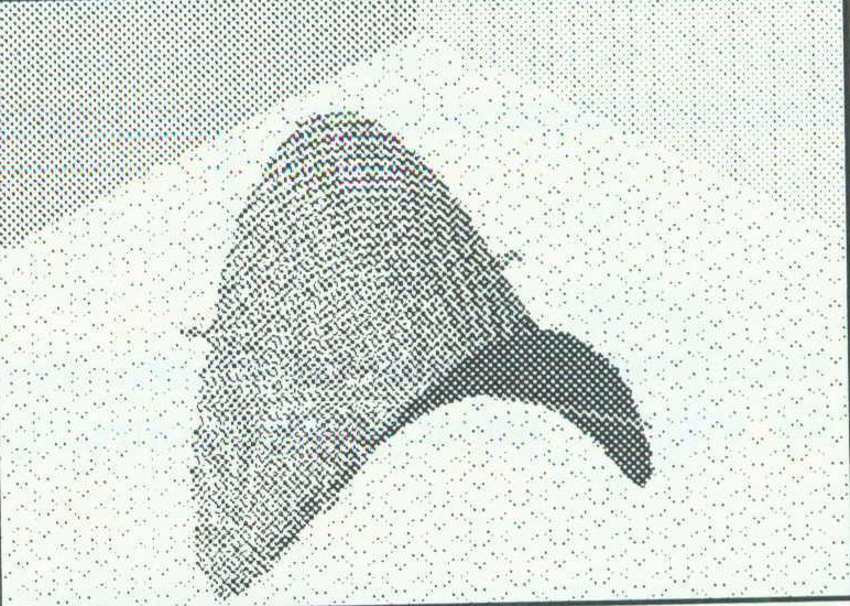
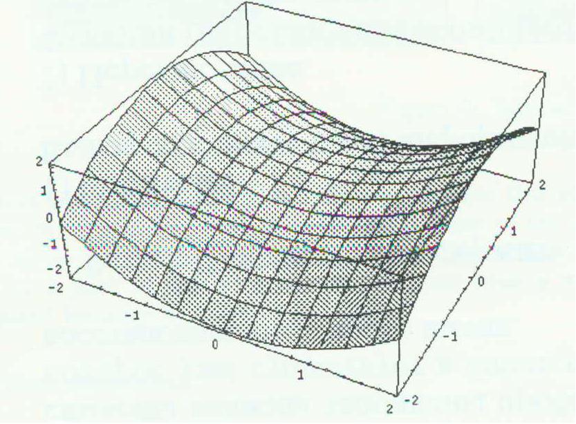
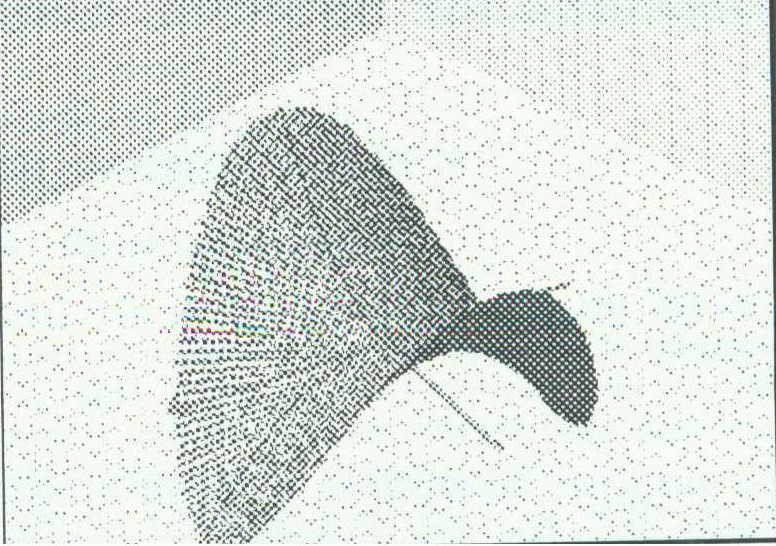
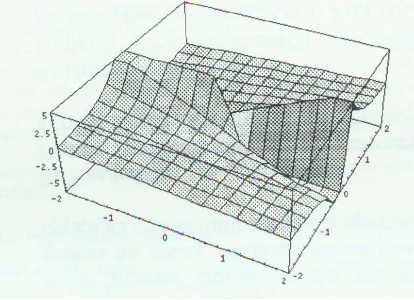
Figure 8: xy, (x²-y²)/2, x/y in the Mathematica (left side) and in the Graphing Calculator (right side)

than leaving it undefined at 0, or returning a Dirac delta function). Obviously, such a simple test is not enough to solve all Obviously, such a simple test is not enough to solve all discontinuity problems. However, for little additional cost when computing points, one systematically can improve the correctness of the surface rendered.

Equivalence of surfaces

     An important concept a plotting system should convey is that of geometrically equivalent and/or similar objects. Consider z=xy, z=(x²-y²)/2, and z=x/y, for example. plotting these equations should produce similar pictures, as the second equation is just a rotation of the first one by п/4 and the third equation is a permutation of x, y, z on the first one (except that the line along the z-axis should be removed in the plot).
     Now consider the left side of Figure 8. It shows the pictures produced by Mathematica for three equations. These pictures look quite different for several reasons. For example, by plotting over a square grid, the curve of intersection between the function z=f(x,y) and the planes of constant x and y at the edge of the graph become features of the surface.
     The right side of figure 8 presents praphs of the same functions in the Graphing Calculator plotted over a circular domain. here it is obvious that the first two surfaces are geometrically equivalent, yet the third still looks dramatically different for three reason: (1) plotting over the domain sqr(x²+y²)<2 automatically bounds |z|<2 for the first two formulas, but not for the third producing a different clipping. Clipping the points so that sqr(x²+y²+z²)<2 would make the images more similar. (2) the used rendering algorithm shades the top and bottom of surfaces differently which results in ambiguities at places where the top and the bottom are indistinguishable. We can observe this effect in figure 8f by noticing that the top and bottom of the surface join along the z-axis. (3) Although only the z-axis should not be a part of this plot, many polygons near y=0 are dropped because of their large z-value.